This article is part of my series of projects around Ternary Computing and Processor Design. Click here to see the list of projects of this series.
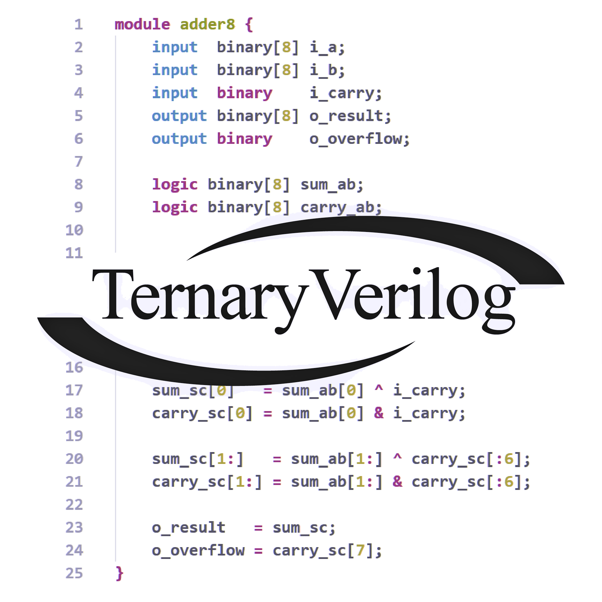
After my internship at Arm, I seeked to improve my hardware design skills through the continuation of my exploration of ternary logic and its application to processor design. However, current Hardware Description Languages (HDL) mostly support binary logic only. Moreover, the tools are very impractical both for development and simulation/debugging. Therefore, I obviously had to develop my own HDL ! (if I don't stop soon, I'll start developing my own operating system...). Anyway, I present to you TernaryVerilog.
In this article, I will first describe the main features of the language, then explain how the tools I developed work, followed by a short documentation of the syntax.
The tools
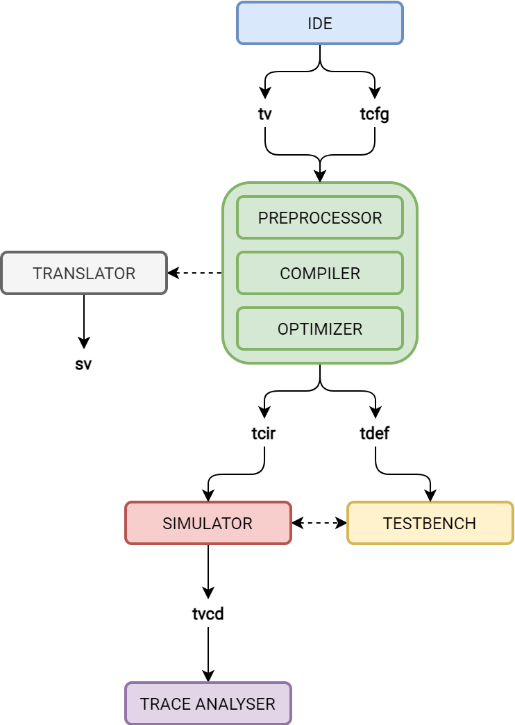
TernaryVerilog development workflow
Compiler-synthesizer
The synthesizer/compiler is coded in Python because performance is not an issue (yet ?) and I wanted to be able to develop this faster. It works using the standard compiler design. Through a command-line interface, the compile options are provided. The compiler takes a single TernaryVerilog file as input. This main file can then include other files. First, if enabled, the file is preprocessed which creates a new version of the file.
   TernaryVerilog Compiler CLI :
tvcompiler FILE [-o|--output OUTPUT_FILE] [-p|--preprocess] [-P|--ppdir PREPROCESSOR_DIRECTORY] [-c|--configs PREPROCESSOR_CONFIGS...] [-T|--templates TEMPLATE_DIRECTORIES...] [-r|--reduced] [-O|--optimized] [-w|--warnings] [-v|--verbose] [-t|--tree]
    FILE path and file name of the main .tv input file to compile
    -o --output OUTPUT_FILE path and file name for the output .tcir and .tdef files
    -p --preprocess enable the preprocessor
    -P --ppdir PREPROCESSOR_DIRECTORY directory where preprocessed files will be written
    -c --configs PREPROCESSOR_CONFIGS... list of config files containing the parameters used by the Jinja2 preprocessor
    -T --templates TEMPLATE_DIRECTORIES... directories of templates used by the Jinja2 preprocessor
    -r --reduced enable reduced output (only reg2reg signals)
    -O --optimized enable circuit optimization
    -w --warnings enable syntax and semantic warning messages
    -v --verbose enable compilation status messages
    -t --tree enable abstract syntax tree message
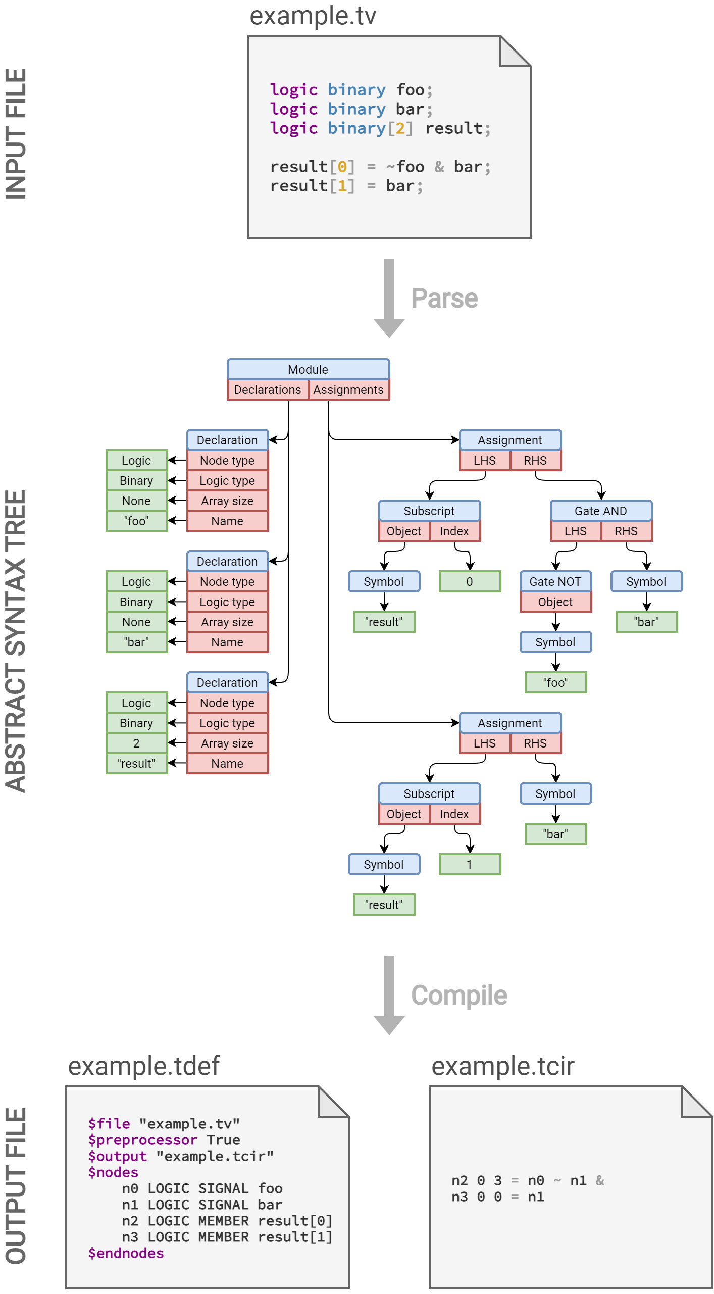
The preprocessed file is then parsed into a list of tokens. Then, the list of tokens is fed to a finite state machine which carries out syntax analysis and outputs an Abstract Syntax Tree (AST) of syntax groups. The shunting yard algorithm is used to convert arithmetic operations into an AST representation. If any syntax errors and warnings are detected, the user is notified. If include statements are detected, the corresponding files are read, tokenized and syntax-analyzed sequentially in order of inclusion. When all files have gone through syntax analysis, the AST is converted through semantic analysis to a synthesized circuit described in a net-gate network. Semantic errors and warnings are detected.
Finally, the circuit is written to two files : a .tcir file listing the nodes by id with all information necessary for the simulator (propagation delay, trigger signal for flip-flops, and of course the expression in Reversed Polish Notation (RPN) with node IDs and gate operators) ; and a .tdef file containing information about compilation, the structure of the circuit, the names of each node with their ID, the structures, arrays and words, and everything else necessary to debug and visualize the circuit during simulation.
Half-adder
Optimizer
Since this article was written, I've worked on a circuit optimizer. When fed a .tcir file, it parses in a AST, counts the number of transistors, measures the latency for every reg2reg path, and calculates the maximum frequency the circuit can run at. It then tries to rewrite the AST while not modifying the functional design in order to reduce both the number of transistors and the maximum latency. Finally, the optimized circuit is re-encoded to .tcir to be used by the simulator. For more details about how the optimizer works and the preliminary results, you can read the article I wrote on the project (WIP).
Simulator
The simulator can be used either manually with Command Line Interface, or connect to a debugging tool such as the Testbench using a Zero-MQ interface. It first reads and parses a .tcir circuit file and for each node it builds a tree of operations (logic gates) with the leaves being other nodes or constant values. Then, it can simulate the circuit either with or without latency simulation : the compiler calculates the latency of each gate based on the depth of the CMOS equivalent gate. Iterating over all nodes, the signals are first updated through simulator input (value injection), then the signals corresponding to registered are updated according to their triggering signal, and then the changes are propagated through the rest of the nodes. Finally, the simulator can return the values of each node to the user or the testbench. Additionally, we can modify the value of each node at any step of the simulation. This is useful to initialize certain parts of the circuit such as memory, or to load a particular step for debugging and fault testing.
After each simulation step, the simulator writes to a custom Value Change Dump file (.tvcd). As the name implies, this file contains the logs of a simulation by storing when each signal changes value and to which logic value. This .tvcd can then be read by another tool to reconstruct the chronogram of each signal during the simulation.
I plan to develop an even more optimized simulator with a novel design I have never tried or seen. The simulator reads the circuit file and builds another C++ file with each signal as a variable. This can remove some overhead left even after GCC optimization and allow for the use of large Look-Up Tables (LUT)for certain multi-input circuits. This will be very useful for fault testing, and when evaluating the performance of more complex processors able to run simple benchmarks over millions of clock cycles.
Testbench
The testbench is a Python library which allows the user to easily interface with the simulator and visualize the state of a circuit. In a Python script, the use can create testbench objects (such as register, clock and memory) and link them to signals of the circuit through the .tdef file generated by the compiler. Those objects then act as interface elements to both initialize the values at the start of the simulation (initialize memory to load a program for instance), control the values during the simulation (to update the clock and define the frequency) and to fetch the results and visualize it in the terminal using UTF box drawing characters and ANSI escape sequences for colors. This tool is useful to quickly test if simple circuit work.
TelociDesi
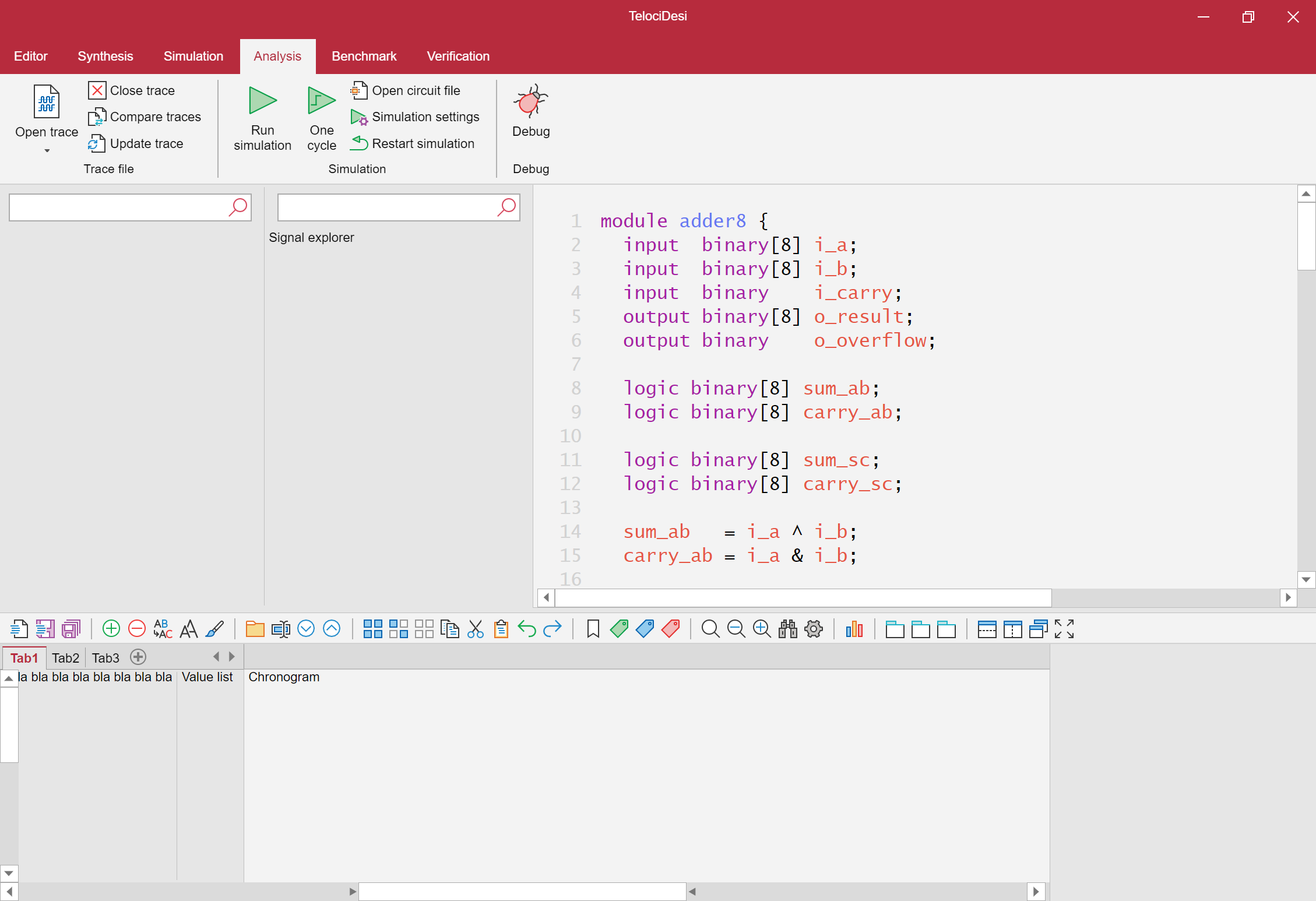
Screenshot of the WIP software
TelociDesi is an Electron-based application to unify all the tools for TernaryVerilog development : coding and synthesizing TernaryVerilog, exploring and debugging the circuits, launching simulations and benchmarks, visualize signal traces, verify the functions of modules, study the impact of design parameters, calculate the maximum frequency of a circuit and identify the critical path, and much more. This project is still in development.
Additional tools
I've also developed a syntax highlighter for Visual Studio Code using RegEx. It is based on the package for SystemVerilog but modified to understand TernaryVerilog syntax. This makes writing TV code much easier. I've planned to develop more utilities such as live linting and auto-completion also for VS Code, as well as their integration into TelociDesi.
Documentation
Signal declaration
Signals are the nets holding a logic value during the simulation. Signals have a name used to reference them in the code, a node type and a logic type. The name must only include alphanumerical characters and underscores (the first character must be a letter or an underscore). The node type describes how the signal connects to other signals and modules. The logic type describes what values the net can hold.
The node type can be one of the following :
logic: structural signal used inside a module or at the global scope, synthesized as a wire.register: behavioral signal used inside a module or at the global scope, synthesized as a flip-flop, can hold a value assigned in a posedge or negedge block with a trigger signal.input: structural signal used to input a value to a module, synthesized as a wire.output: structural signal used to output a value from a module, synthesized as a wire.pinin: equivalent to logic, should be used for interface signals with the testbench.pinout: equivalent to logic, should be used for interface signals with the testbench.
The logic type can be one of the following :
binary: single binary signal, can hold the values 0, 1 and x (undefined).ternary: single ternary signal, can hold the values -1, 0, 1 and x (undefined).- A custom struct : aggregate object of other signals as defined in a struct block.
Additionally, square brackets are used to indicate that the signal is an array. ternary[9] creates a one-dimensional word of 9 ternary signals (addressed from 0 to 8). binary[4][16] creates a two-dimensional array of 16 words of 4 binary signals (addressed first from 0 to 15, and then from 0 to 3). Arrays of more than two dimensions are not supported yet. One-dimensional arrays of structures are also possible : mystruct[3] creates an array of 3 objects of type mystruct (addressed from 0 to 2). Arrays are indexed LSD (Least Significant Digit) first : arr[0] is the least significant bit of the array ; it is also the rightmost bit, this is important for the concatenation operator explained later.
Examples of signal declarations :
input binary clk;
input mystruct[3] i_data;
output ternary[3] o_result;
register binary[8][16] r_memory;
logic binary[16] pointer;
logic ternary flag_sign;
pinout binary[4] ext_device_id;
pinin binary[4] ext_bus;
Multiple declarations in a single line with a comma-separated list of signal names is planned but not yet implemented.
Structures
Structures are aggregate objects of multiple signals of any type. Structures are declared at the global scope of any file. Each structure must be given a unique name by which it is referenced for signal declarations. Since all files are parsed before syntax analysis, structures can be declared anywhere before or after being referenced in a signal declaration and cannot be scoped to one file only. A structure is declared using the struct keyword :
struct MyStruct {
    binary attribute;
    ternary[3] word_attr;
    binary[4][16] array_attr;
    OtherStruct struct_attr;
    OtherStruct[2] struct_array_attr;
}
Instances of a structure are declared as explained in the signal assignment section above. Structure attributes are accessed and assigned using the member access operator (dot) as explained in the signal assignment section below.
Combinatorial signal assignment
Combinational assignments are always active and correspond to a gate-level description of the circuit. The syntax used is simply LHS = RHS; at the root of the main file or in a module declaration. Each signal should only be assigned once. If a signal is assigned multiple times, the compiler will throw a warning. Circular assignments are not allowed and the compiler will throw an error. The LHS expression can use the subscript operator or the member access operator. The RHS expression combines operands with appropriate operators to produce the desired functional expression using any of the operators detailed below.
For all examples below, a, b, c and d are singular signals which can be written as 1D arrays of size 1 {a}, {b}, {c} and {d} respectively ; u, v and w are 3-elements words which can be written as 1D arrays of size 3 {u2,u1,u0}, {v2,v1,v0} and {w2,w1,w0} respectively ; t is an array of two rows and three columns (array of two words each of size three) flattened to {t1,2,t1,1,t1,0,t0,2,t0,1,t0,0} ; s is a structure instance of type MyStruct as defined above.
Duoary operators perform an operation on two operands placed on either sides. The operands must be homogenous in size and should be homogenous in logic type All duoary operators are applied bit-wise on arrays. Note that the expression "duoary operator" is a neologism used instead of "binary operator" to not be confused with operators applied to binary or ternary signals.
| Operator | Symbol | Example |
|---|---|---|
| Binary AND | & |
a&b describes {a&b} v&w describes {v2&w2 , v1&w1 , v0&w0} |
| Binary OR | | |
a|b describes {a|b} v|w describes {v2|w2 , v1|w1 , v0|w0} |
| Binary XOR | ^ |
a^b describes {a^b} v^w describes {v2^w2 , v1^w1 , v0^w0} |
| Ternary AND | × |
a×b describes {a×b} v×w describes {v2×w2 , v1×w1 , v0×w0} |
| Ternary OR | + |
a+b describes {a+b} v+w describes {v2+w2 , v1+w1 , v0+w0} |
| Ternary CONS | ⊠ |
a⊠b describes {a⊠b} v⊠w describes {v2⊠w2 , v1⊠w1 , v0⊠w0} |
| Ternary ANY | ⊞ |
a⊞b describes {a⊞b} v⊞w describes {v2⊞w2 , v1⊞w1 , v0⊞w0} |
| Ternary MUL | ⊗ |
a⊗b describes {a⊗b} v⊗w describes {v2⊗w2 , v1⊗w1 , v0⊗w0} |
| Ternary SUM | ⊕ |
a⊕b describes {a⊕b} v⊕w describes {v2⊕w2 , v1⊕w1 , v0⊕w0} |
Unary operators perform an operation on one operand. The operator is said prefix if it is placed before the operand, and postfix if it is placed after. For an array operand, the operand is said to distribute bit-wise when it is applied to each element of the array and results in an array of the same size, and is said to distribute by reduction when it is applied to the array as a whole and results in a single signal. Duoary operators can be used as unary operators forming a reduction functional group.
| Operator | Symbol | Placement | Distribution | Example |
|---|---|---|---|---|
| Binary NOT | ~ |
Prefix | Bit-wise | ~a describes {~a} ~w describes {~w2 , ~w1 , ~w0} |
| Ternary NOT | ¬ |
Prefix | Bit-wise | ¬a describes {¬a} ¬w describes {¬w2 , ¬w1 , ¬w0} |
| Ternary PNOT | ⊤ |
Prefix | Bit-wise | ⊤a describes {⊤a} ⊤w describes {⊤w2 , ⊤w1 , ⊤w0} |
| Ternary NNOT | ⊥ |
Prefix | Bit-wise | ⊥a describes {⊥a} ⊥w describes {⊥w2 , ⊥w1 , ⊥w0} |
| Ternary ISP | ⁺ |
Postfix | Bit-wise | a⁺ describes {a⁺} w⁺ describes {w2⁺ , w1⁺ , w0⁺} |
| Ternary ISZ | ⁰ |
Postfix | Bit-wise | a⁰ describes {a⁰} w⁰ describes {w2⁰ , w1⁰ , w0⁰} |
| Ternary ISN | ⁻ |
Postfix | Bit-wise | a⁻ describes {a⁻} w⁻ describes {w2⁻ , w1⁻ , w0⁻} |
| Binary AND | & |
Prefix | Reduction | &w describes {w2 & w1 & w0} |
| Binary OR | | |
Prefix | Reduction | |w describes {w2 | w1 | w0} |
| Binary XOR | ^ |
Prefix | Reduction | ^w describes {w2 ^ w1 ^ w0} |
| Ternary AND | × |
Prefix | Reduction | ×w describes {w2 × w1 × w0} |
| Ternary OR | + |
Prefix | Reduction | +w describes {w2 + w1 + w0} |
| Ternary CONS | ⊠ |
Prefix | Reduction | ⊠w describes {w2 ⊠ w1 ⊠ w0} |
| Ternary ANY | ⊞ |
Prefix | Reduction | ⊞w describes {w2 ⊞ w1 ⊞ w0} |
| Ternary MUL | ⊗ |
Prefix | Reduction | ⊗w describes {w2 ⊗ w1 ⊗ w0} |
| Ternary SUM | ⊕ |
Prefix | Reduction | ⊕w describes {w2 ⊕ w1 ⊕ w0} |
The conditional operator describes a multiplexer. The first operand is the condition, followed by two or three operands called paths. The syntax uses the ? symbol after the condition and the : symbol to separate the paths. If the condition is a binary signal, it expects two paths, respectively for logic values $$1$$ and $$0$$ ; and if the condition is a ternary signal it expects three paths, respectively for logic values $$+$$, $$0$$ and $$-$$. A ternary condition can be used with binary paths and vice-versa, as long as the paths are homogenous in logic type. The paths can be singular signals, words, arrays or structures as long as they are homogenous in size. If the condition is a word or array instead of a singular signal, and homogenous in size with the operands, then the conditional operator is applied bit-wise. Examples of conditional operators and their resulting signal :
a ? b : c with a a binary signal describes {a?b:c}
|
a ? b : c : d with a a ternary signal describes {a?b:c:d}
|
a ? v : w with a a binary signal describes {a?v2:w2 , a?v1:w1 , a?v0:w0}
|
u ? v : w with u a word of binary signals describes {u2?v2:w2 , u1?v1:w1 , u0?v0:w0}
|
The concatenation operator combines singular signals or words into words. The syntax for a concatenation functional group is a list of , comma-separated operands inside {} curly brackets. The order is important as the left most operand corresponds to MSDs (Most Significant Digits) and the rightmost operand corresponds to LSDs (Least Significant Digits). Remember that words and arrays are indexed LSB-first, hence rightmost-first. Note that while using arrays or structures in concatenation works, and flattens the signals into a word (row-after-row for arrays, and with the attributes of the structures concatenated in order of the structure declaration), it is not recommended for readability reasons. Examples of concatenation and the resulting signals :
{a,b,c} describes {a,b,c}
|
{a,w} describes {a,w2,w1,w0}
|
{w,a} describes {w2,w1,w0,a}
|
{v,w} describes {v2,v1,v0,w2,w1,w0}
|
The vectorization operator repeats a singular signal or a word into a longer word of a given size. The syntax for a vectorization functional group is the size of the desired resulting signal, followed by the ' apostrophe symbol, and finally the signal to vectorize. Examples of vectorization and the resulting signals :
3'a describes {a,a,a}
|
6'w describes {w2,w1,w0,w2,w1,w0}
|
4'w describes {w0,w2,w1,w0}
|
2'w describes {w1,w0}
|
5'{a,b} describes {b,a,b,a,b}
|
Subscripting is used to access elements of words and arrays. The syntax for subscripting is the object to subscript, followed by the indexing in [] square brackets. The indexing can be element-based with a single number, or ranged with a : colon separating the start index on the left and end index on the right. In the case of element indexing, the result is a singular signal when subscripting a word, and a word when subscripting an array. In the case of ranged indexing, the result is a sub-word when subscripting a word, and a sub-array when subscripting an array. Indexing starts at 0 for the first element, which corresponds to the LSD and rightmost element. A negative index starts with the last element and counts backwards. An index greater than the size of the object wraps around (the index is modulo the size of the object). In the case of ranged indexing, if the start index (on the left) if greater than the end index (on the right), the elements of the result are in opposite order to the original object. In the case of ranged indexing, the start or end index can be omitted and will default to the start or end of the object respectively. Examples of subscripting :
w[0] describes {w0}
|
w[1] describes {w1}
|
w[-1] describes {w2}
|
w[3] describes {w0}
|
w[0:1] describes {w1,w0}
|
w[1:] describes {w2,w1}
|
w[:1] describes {w1,w0}
|
w[2:0] describes {w0,w1,w2}
|
w[-1:0] describes {w0,w1,w2}
|
{a,b,c}[0] describes {c}
|
The member access operator is used to assign and access attributes of a structure. The syntax is the instance of a structure, followed by the . symbol and finally the name of the attribute to access. In the future, this operator will also be used to access input and output signals of module instances, but this feature is not implemented yet. Examples of member access :
s.attribute
|
s.word_attr[2]
|
s.struct_attr.var
|
s.struct_array_attr[0].var
|
Finally, constants (hardcoded values) can be used in expressions, either binary or ternary, and in many encodings. The syntax for a constant is the following : the number of digits of the constant, then the encoding of the constant, then the $ symbol, then the value of the constant with the appropriate encoding. The encoding is noted with letters describing the logic encoding and and optional base encoding. The logic encodings are : b for binary (0 and 1), t for balanced ternary (0, 1 and i for -1), and u for unbalanced ternary (0,1 and 2) coded in balanced ternary ($$u0=t-$$, $$u1=t0$$ and $$u2=t+$$). The base encodings are : d for decimal (0 to 9), x for hexadecimal (0 to f), o for octal (0 to 7), h for heptavintinal (0 to z by skipping certain letters as described by Douglas W. Jones), n for nonal (0 to 8). Underscores can be used when writing the value of the constant as a separator. Signed binary constants are not yet implemented and must be written manually. Examples of constants :
1b$0 describes {0}
|
4b$0101 describes {0,1,0,1}
|
8b$0101_1100 describes {0,1,0,1,1,1,0,0}
|
3t$01i describes {0,+,-}
|
3u$012 describes {-,0,+}
|
4bd$13 describes {1,1,0,1}
|
6bo$27 describes {0,1,0,1,1,1}
|
8bx$4f describes {0,1,0,0,1,1,1,1}
|
5td$19 describes {0,+,-,0,+}
|
3tn$6 describes {+,-,0}
|
3tn$-8 describes {-,0,+}
|
Missing operators
Note that there are missing operators compared to other Hardware Description Languages or programming languages.
First, expressions that are not practically synthesizable such as dynamic subscripting a[b] and dynamic-size vectorization a'b are not possible.
Shift operations can be easily expressed with subscripting and concatenation :
| Shifting | Fill | Expression | Result |
|---|---|---|---|
| $$w<<1$$ | Padding | {w[0:1],1b&0} |
{w1,w0,0} |
| $$w<<1$$ | Wrapping | {w[0:1],w[-1]} |
{w1,w0,w2} |
| $$w>>1$$ | Padding | {1b&0,w[1:]} |
{0,w2,w1} |
| $$w>>1$$ | Wrapping | {w[0],w[1:]} |
{w0,w2,w1} |
Word-wise arithmetic operations (add, subtract, multiply, divide, modulo, power, increment, decrement) are complex in hardware and there exists many implementations (such as ripple-carry adder and carry-lookahead adder) with different properties (latency, size, etc). Therefore, those operations should be implemented through a custom module. TernaryVerilog is therefore closer to circuit description than Verilog which is more abstract and leaves more of the work to the synthesizer. For the same reason, comparisons (greater than, greater or equal to, less than, less or equal to) are not available. The comparisons equal and not-equal are easy enough to implement with gates.
Synchronous signal assignment
Register assignments are described with synchronous assignment blocks using the posedge or negedge keyword for rising-edge-triggered or falling-edge-triggered flip-flops, followed by the trigger signal. Multiple synchronous assignments can be written implemented in a synchronous assignment block. Example of the syntax :
pinin binary clk;
logic binary a;
logic binary b;
register binary res1;
register binary res2;

posedge clk {
    res1 = a & b;
    res2 = a | b;
}
Note that the trigger signal cannot be an expression such as clk & reset or triggers[0]. If this is necessary, a separate logic signal should be declared and assigned then used as a trigger.
Note that circular assignments with the previous value of the register inside the synchronous assignment block are not allowed, that each register can be assigned in only one synchronous assignment block even with different trigger signals, and that there is no if-else syntax. Those restrictions exist to make the code easier to read and to make compilation much easier. The recommended workaround is to declare and assign a logic signal for the next value of the register. For example, if a register res is triggered by the rising edge of the clock signal clk, needs to be initialized to $$0$$ when the reset control signal is true, and updated to the value of $$a|b$$ if the enable signal en is true, else it keeps its previous value :
pinin    binary clk;
pinin    binary reset;
logic    binary en;
logic    binary a;
logic    binary b;
register binary res;
logic    binary next_res;

next_res = reset ? 1b$0
            : en ? (a | b)
                 : res;

posedge clk {
    res = next_res;
}
Modules and instantiation
A module is a circuit with input, outputs and internal signals with their assignments. Modules are used for code factorization, abstraction and structuring. Similar to a class in programming languages, a module needs to be declared, then any number of instances of the module can be created.
A module is declared with the module keyword followed by the name of the module and the block containing all the signal declarations and assignments. Input and output signals are declared like regular signals using the input and output keywords. They can be declared anywhere in the code but it is recommended to declare them at the top of the module. Assignments inside the module can only use the signals declared inside the module and the input and output signals of the module. The module can also include instances of other modules and synchronous assignment blocks.
Instance of a module are create using the instance keyword, followed by the name of the module, then by the unique name of the instance, and finally the block of connections. Connections describe how the input and output signals of the instance of the module connect to signals outside the module. Connections work like regular assignments, with a . symbol at the start of the line, thus they support RHS expressions with operations.
Here is an example of two module declarations, with one module instantiated inside the other.
module MyFirstModule {
    input  binary clk;
    input  binary i_a;
    input  binary i_b;
    output binary o_q;

    logic binary c;

    c = a & b;
    o_q = ~c;
}

module MySecondModule {
    input  binary    clk;
    input  binary    reset;
    input  binary[2] i_w;
    output binary    o_res;

    logic    binary n_res;
    register binary   res;

    logic binary q;
    instance MyFirstModule firstInstance {
        .clk = clk;
        .i_a = i_w[0];
        .i_b = i_w[1];
        .o_q = q;
    }

    n_res = reset ? 1b$0 : q;
    posedge clk {
        res = n_res;
    }
    o_res = res;
}

pinin binary    clk;
pinin binary    reset;
logic binary[2] v;
logic binary    result;

instance MySecondModule mainInstance {
    .clk   = clk;
    .reset = reset;
    .i_w   = v;
    .o_res = result;
}
File structure
The compiler takes a single source file as argument, the main TernaryVerilog file. However, a project can be broken down into many files in two ways : preprocessor includes and compilation includes.
The former uses the Jinja2 include preprocessor statement and is equivalent to copy-pasting the content of one file into another. Therefore, a single TV file is generated. This method also allows for including code anywhere : inside module declarations, even in assignment statements. Moreover, using the with preprocessor statement, we can pass parameter values to the included code, thus allowing for templates. This is explained in more details in the preprocessor section.
The latter uses include statements at the root of the file, preferably at the top for readability. The file included is pushed to the compilation list. The files in the list are compiled sequentially in-order. Example :
// file2.tv
struct MyStruct {
    binary attr;
}
// main.tv
include "file2.tv";
logic MyStruct s;
As the compiler works by stages with global variables and doesn't care about order of declaration (only scope is important), using both methods, a module or structure declared in one file is accessible in all files.
Preprocessor
The preprocessor uses the Jinja2 framework and syntax. When compiling a TernaryVerilog project, if the preprocessor is enabled, config files can be provided to define constants used by the preprocessor. Those config files use the .tcfg extension but are equivalent to Python scripts as described in the Jinja2 documentation. Therefore Python functions can be used including libraries and file input.
For more information about Jinja2 preprocessing, please refer to Jinja2's documentation. Here are some simple examples of preprocessing :
// parameters.tcfg
PARAM_VAR = 5
PARAM_LIST = range(PARAM_VAR)
PARAM_BOOL = True
// main.tv
logic binary a;
logic binary b;
logic binary[{{PARAM_VAR}}] q;

b = {%if PARAM_BOOL%} 1b$0 {%else%} a {%endif%};

{%for idx in PARAM_LIST%}
logic binary res_{{idx}};
res_{{idx}} = q[{{idx}}] & b;
{%endfor%}
// main.tv after preprocessing
logic binary a;
logic binary b;
logic binary[5] q;

b = 1b$0;

logic binary res_0;
res_0 = q[0] & b;
logic binary res_1;
res_1 = q[1] & b;
logic binary res_2;
res_2 = q[2] & b;
logic binary res_3;
res_3 = q[3] & b;
logic binary res_4;
res_4 = q[4] & b;
This article is part of my series of projects around Ternary Computing and Processor Design. Click here to see the list of projects of this series.
Go back to the list of projects